The Equichordal Point Problem
A recent major result of Marek Rychlik is a solution of the Equichordal Point Problem. This result has been published in Inventiones Mathematicae, 129(1), pp. 141-212, 1997. This famous problem in geometry was posed in 1916 by Fujiwara and in 1917 by Blaschke et. al. and has been attacked by scores of mathematicians over 80 years of its history. The problem can be formulated in simple geometric terms:
A point P inside a closed convex curve C is called equichordal if every chord of C drawn through point P has the same length. Is there a curve with two equichordal points?
It has been conjectured for a long time that a curve with two equichordal points cannot exist. But let us suppose for a moment that such a curve does exist. We will call this curve an equichordal curve. The distance between the potential two equichordal points is called the excentricity of the equichordal curve and will be denoted by a.
If such a curve existed then it would be a union of the two curves depicted in the following motion picture for excentricities varying in the range [.8,.4]:
The two curves are invariant under a map T of the plane into itself defined by the following rule in terms of the two potential equichordal points O1 and O2:
If you are at point P, walk in the direction of O1 by distance 1; when you are done, walk in the direction of O2 by distance 1. The final point Q of your trip is the image of P under T, i.e. Q=T(P).
If the coordinates are chosen so that O1=(-b,0) and O2=(b,0), where b is a half of the excentricity (as in the above movie) then the two curves are unique analytic curves invariant under T and passing throuh points (-1/2,0) and (1/2,0) respectively, and not equal to the x-axis (which is also invariant).
Although numerical studies indicate clearly that the union of these two curves is not a Jordan curve, the solution of the Equichordal Point Problem for all excentricities in the range (0,1) takes about 70 journal pages.
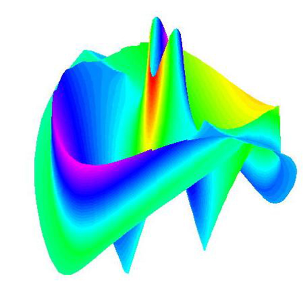
It proves that the problem reduces to studying properties of the following functional equation:
1/( f(m z) – f(z) ) + 1/( f(z) – f(z/m) ) = (1/a) (1 + f(z)^2)^(-1/2)
for a complex function f(z). Here m is a parameter determined from the equation m=(1+a)/(1-a)
This function should have a simple pole at 0 and it is multi-valued. Its meromorphic continuation can be found from the above equation. The following picture is obtained if one plots |f(z)|. The color is determined by Re(f(z)).